Confirmed cases bar graph
# Librerías a utilizar
library(tidyverse)
library(gganimate)
library(readxl)
# Cargo los datos a trabajar
cs_export <- read_excel("cs_export.xls") %>% print()
## # A tibble: 687 x 8
##    `Fecha declarac~ Territorio `Confirmados PC~ Hospitalizados   UCI Curados
##    <chr>            <chr>                 <dbl>          <dbl> <dbl>   <dbl>
##  1 22/05/2020       Andalucía                 9              6     0      26
##  2 22/05/2020       Almería                   1              2     0       4
##  3 22/05/2020       Córdoba                   0              0     0       1
##  4 22/05/2020       Granada                   0              1     0      11
##  5 22/05/2020       Huelva                    1              1     0       0
##  6 22/05/2020       Jaén                      5              2     0       1
##  7 22/05/2020       Málaga                    2              0     0       5
##  8 22/05/2020       Sevilla                   0              0     0       4
##  9 21/05/2020       Andalucía                16              5     0      52
## 10 21/05/2020       Almería                   0              0     0       4
## # ... with 677 more rows, and 2 more variables: Defunciones <dbl>, `Total
## #   confirmados (PCR+test)` <dbl>
# proceso los datos a utlizar
confirmados <-
 cs_export %>%
  group_by(Territorio, `Fecha declaración`)%>%
  print()
## # A tibble: 687 x 8
## # Groups:   Territorio, Fecha declaración [686]
##    `Fecha declarac~ Territorio `Confirmados PC~ Hospitalizados   UCI Curados
##    <chr>            <chr>                 <dbl>          <dbl> <dbl>   <dbl>
##  1 22/05/2020       Andalucía                 9              6     0      26
##  2 22/05/2020       Almería                   1              2     0       4
##  3 22/05/2020       Córdoba                   0              0     0       1
##  4 22/05/2020       Granada                   0              1     0      11
##  5 22/05/2020       Huelva                    1              1     0       0
##  6 22/05/2020       Jaén                      5              2     0       1
##  7 22/05/2020       Málaga                    2              0     0       5
##  8 22/05/2020       Sevilla                   0              0     0       4
##  9 21/05/2020       Andalucía                16              5     0      52
## 10 21/05/2020       Almería                   0              0     0       4
## # ... with 677 more rows, and 2 more variables: Defunciones <dbl>, `Total
## #   confirmados (PCR+test)` <dbl>
almeria <- confirmados %>% filter(Territorio=="Almería")
almeriaacum <- colSums(almeria[3:8])
cadiz <- confirmados %>% filter(Territorio=="Cádiz")
cadizacum <- colSums(cadiz[3:8])
cordoba <- confirmados %>% filter(Territorio=="Córdoba")
cordobaacum <- colSums(cordoba[3:8])
granada <- confirmados %>% filter(Territorio=="Granada")
granadaacum <- colSums(granada[3:8])
huelva <- confirmados %>% filter(Territorio=="Huelva")
huelvaacum <- colSums(huelva[3:8])
jaen <- confirmados %>% filter(Territorio=="Jaén")
jaenacum <- colSums(jaen[3:8])
malaga <- confirmados %>% filter(Territorio=="Málaga")
malagaacum <- colSums(malaga[3:8])
sevilla <- confirmados %>% filter(Territorio=="Sevilla")
sevillaacum <- colSums(sevilla[3:8])
dfaux <- data.frame("Provincia"=c("Sevilla","Málaga","Jaén","Huelva","Granada","Córdoba","Cádiz","Almería"),"ConfirmadosAcum"=c(sevillaacum[6],malagaacum[6],jaenacum[6],huelvaacum[6],granadaacum[6],cordobaacum[6],cadizacum[6],almeriaacum[6]))
# genero el gráfico estático
plot_conf <-
ggplot(dfaux,
aes(x = dfaux$ConfirmadosAcum,
y = dfaux$Provincia,
colour = as.factor(dfaux$Provincia),
fill = as.factor(dfaux$Provincia))) +
geom_bar(stat = "identity",position="stack") +
scale_x_continuous(breaks = seq(500, 5000, 500), expand = c(0,0)) +
theme_bw() +
theme(axis.title = element_blank(),
axis.ticks.y = element_blank(),
legend.position = "none",
panel.grid.minor = element_blank(),
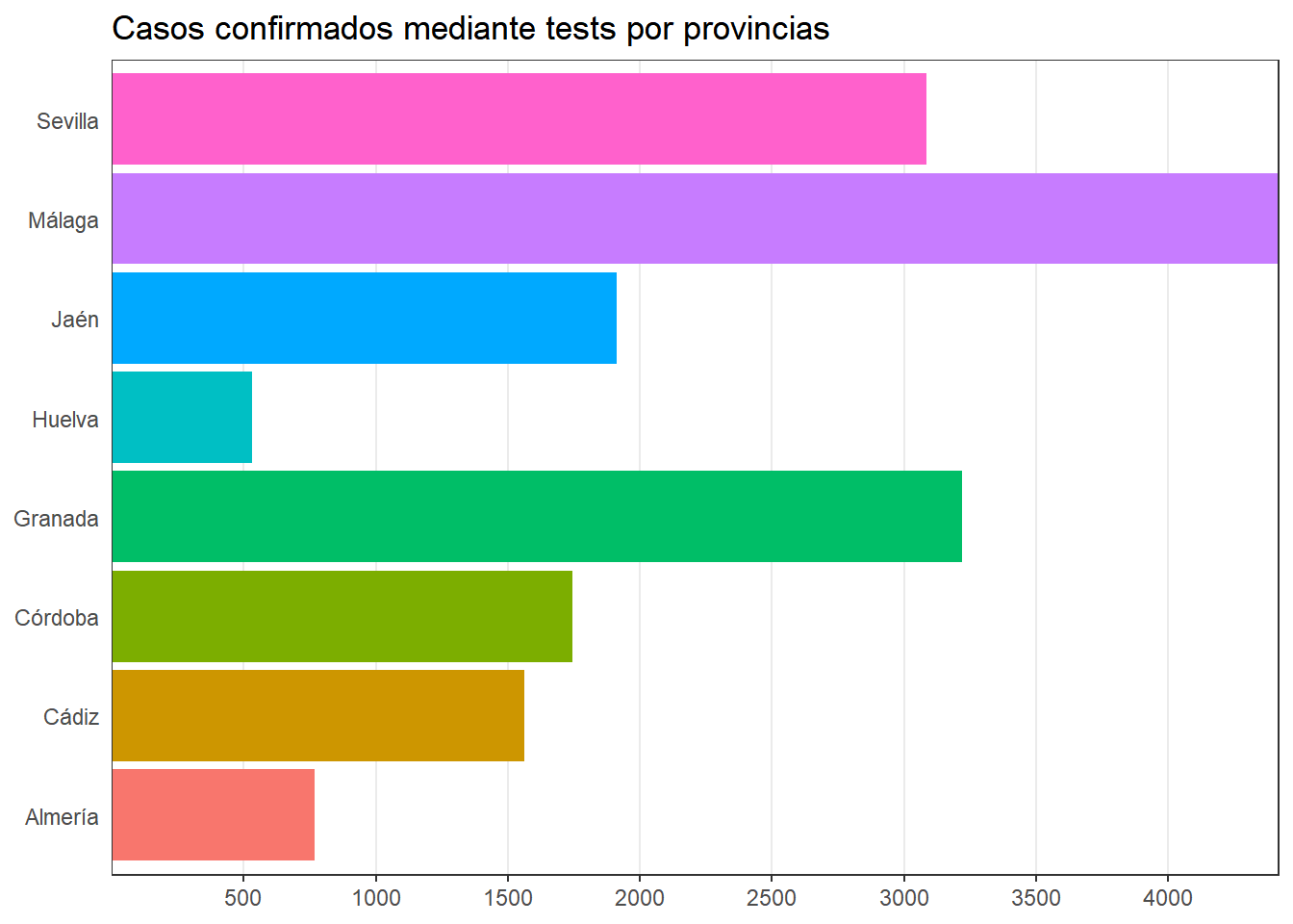
panel.grid.major.y = element_blank())+ggtitle("Casos confirmados mediante tests por provincias")
plot_conf
Andalusia bar graphs
library(readxl)
library(dplyr)
library(ggplot2)
library(lubridate)
library(openair)
library(lattice)
cs_export <- read_excel("cs_export.xls")
filasandalucia <- filter(cs_export, Territorio=="Andalucía" )
aux <- filasandalucia
fechas <- as.Date(aux$`Fecha declaración`,"%d/%m/%Y")
aux$`Fecha declaración` <- sort(fechas)
c <- aux$Curados
h <- aux$Hospitalizados
d <- aux$Defunciones
uci <- aux$UCI
conf <- aux$`Confirmados PCR`
totalconf <- aux$`Total confirmados (PCR+test)`
salidac <- vector("numeric",length(c))
salidah <-vector("numeric",length(h))
salidad <- vector("numeric",length(d))
salidauci <- vector("numeric",length(uci))
salidaconf <- vector("numeric",length(conf))
salidatotalconf <- vector("numeric",length(totalconf))
for(i in seq_along(c)){
salidac[length(c)+1-i] <- c[i]
salidah[length(h)+1-i] <- h[i]
salidad[length(d)+1-i] <- d[i]
salidauci[length(uci)+1-i] <- uci[i]
salidaconf[length(conf)+1-i] <- conf[i]
salidatotalconf[length(totalconf)+1-i] <- totalconf[i]
}
aux$Curados <- salidac
aux$Hospitalizados <- salidah
aux$Defunciones <- salidad
aux$UCI <- salidauci
aux$`Confirmados PCR` <- salidaconf
aux$`Total confirmados (PCR+test)` <- salidatotalconf
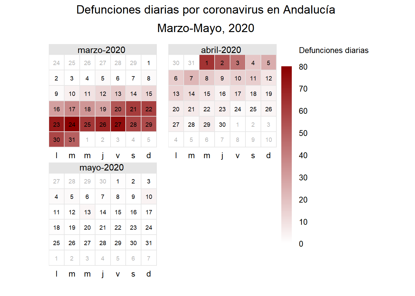
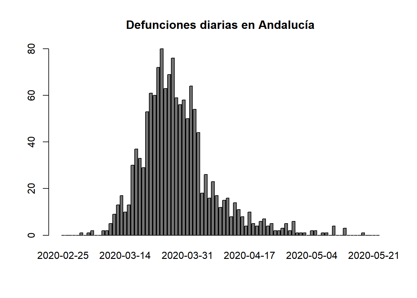
barplot(names.arg=aux$`Fecha declaración`,aux$Defunciones,main="Defunciones diarias en Andalucía",col="grey45")
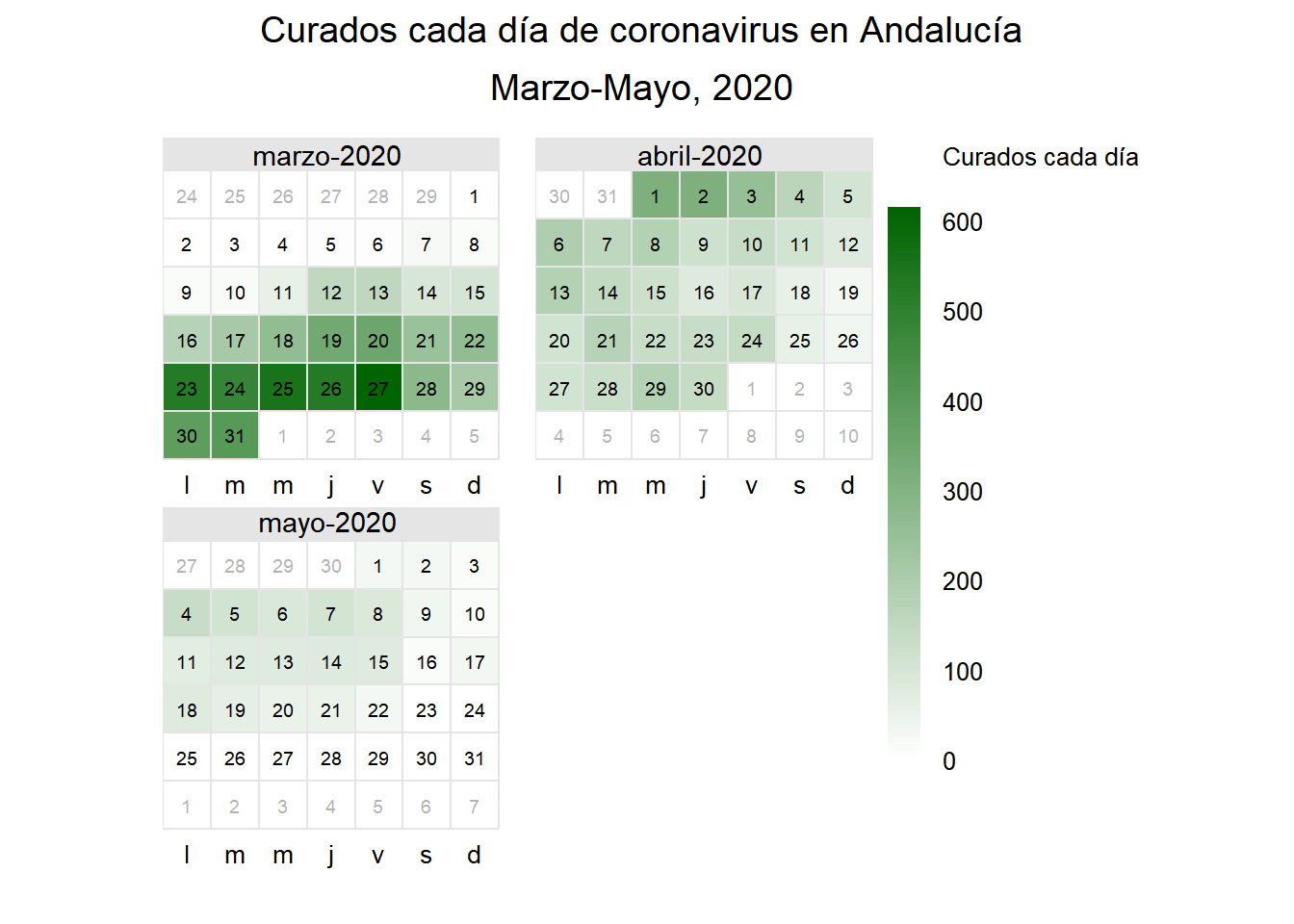
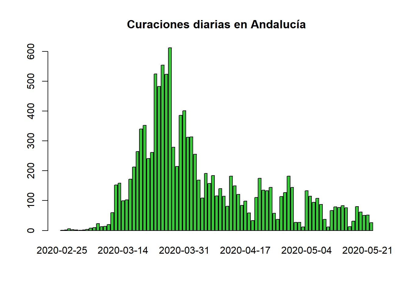
barplot(names.arg=aux$`Fecha declaración`,aux$Curados,main="Curaciones diarias en Andalucía",col="limegreen")
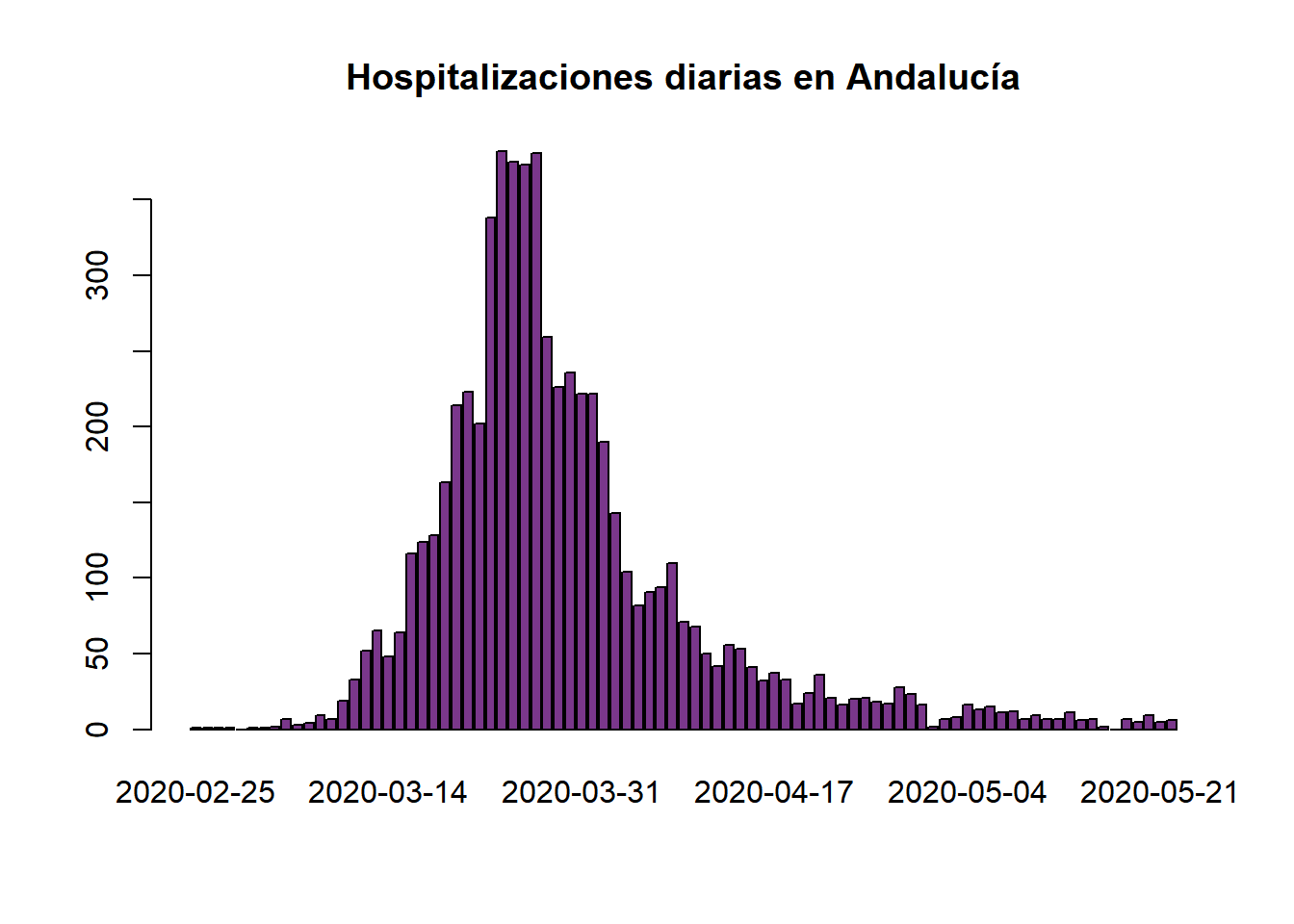
barplot(names.arg=aux$`Fecha declaración`,aux$Hospitalizados,main="Hospitalizaciones diarias en Andalucía",col="mediumorchid4")
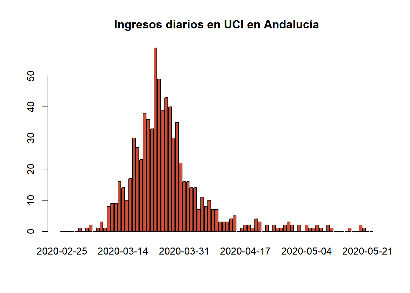
barplot(names.arg=aux$`Fecha declaración`,aux$UCI,main="Ingresos diarios en UCI en Andalucía",col="tomato3")
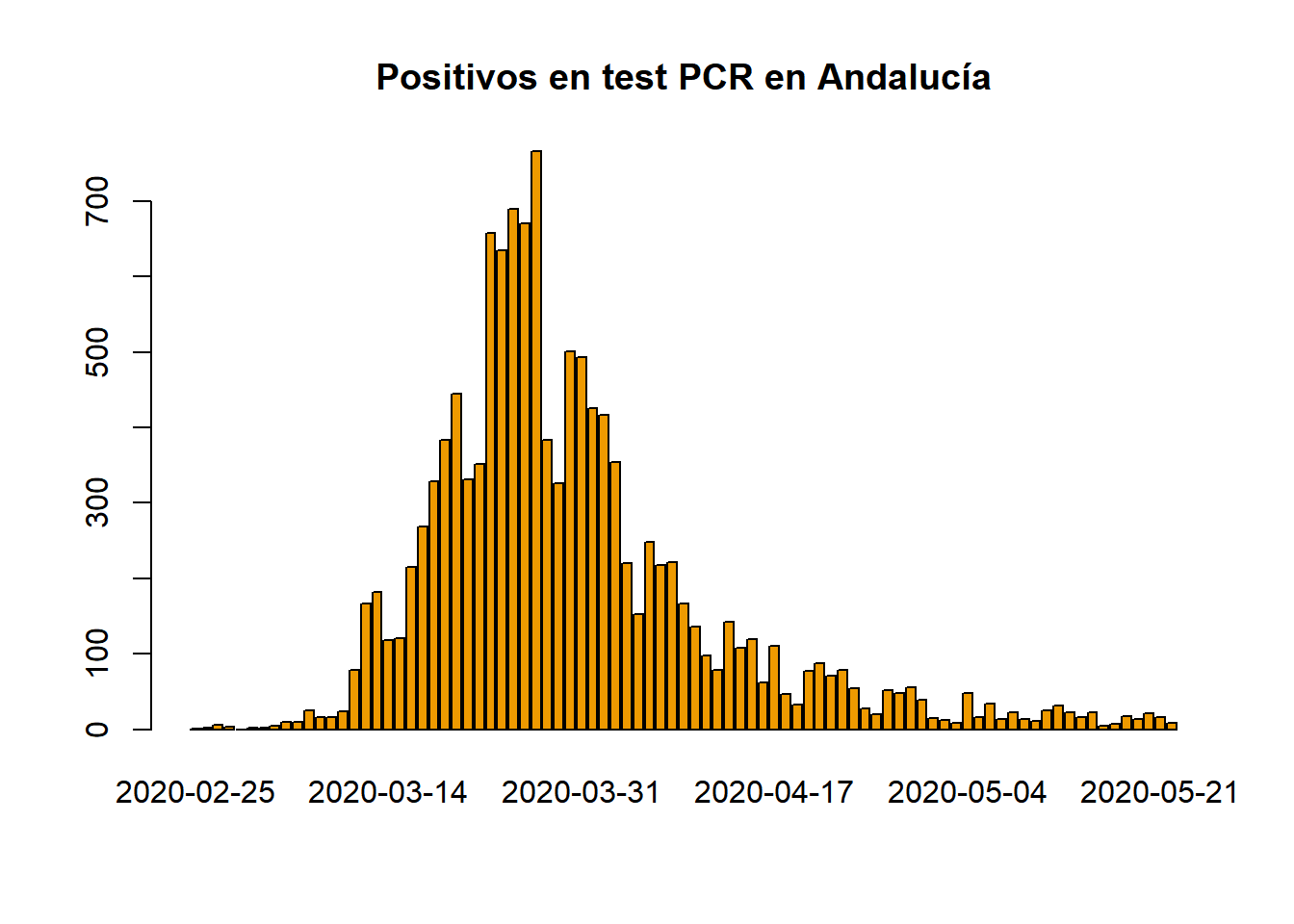
barplot(names.arg=aux$`Fecha declaración`,aux$`Confirmados PCR`,main="Positivos en test PCR en Andalucía",col="orange2")
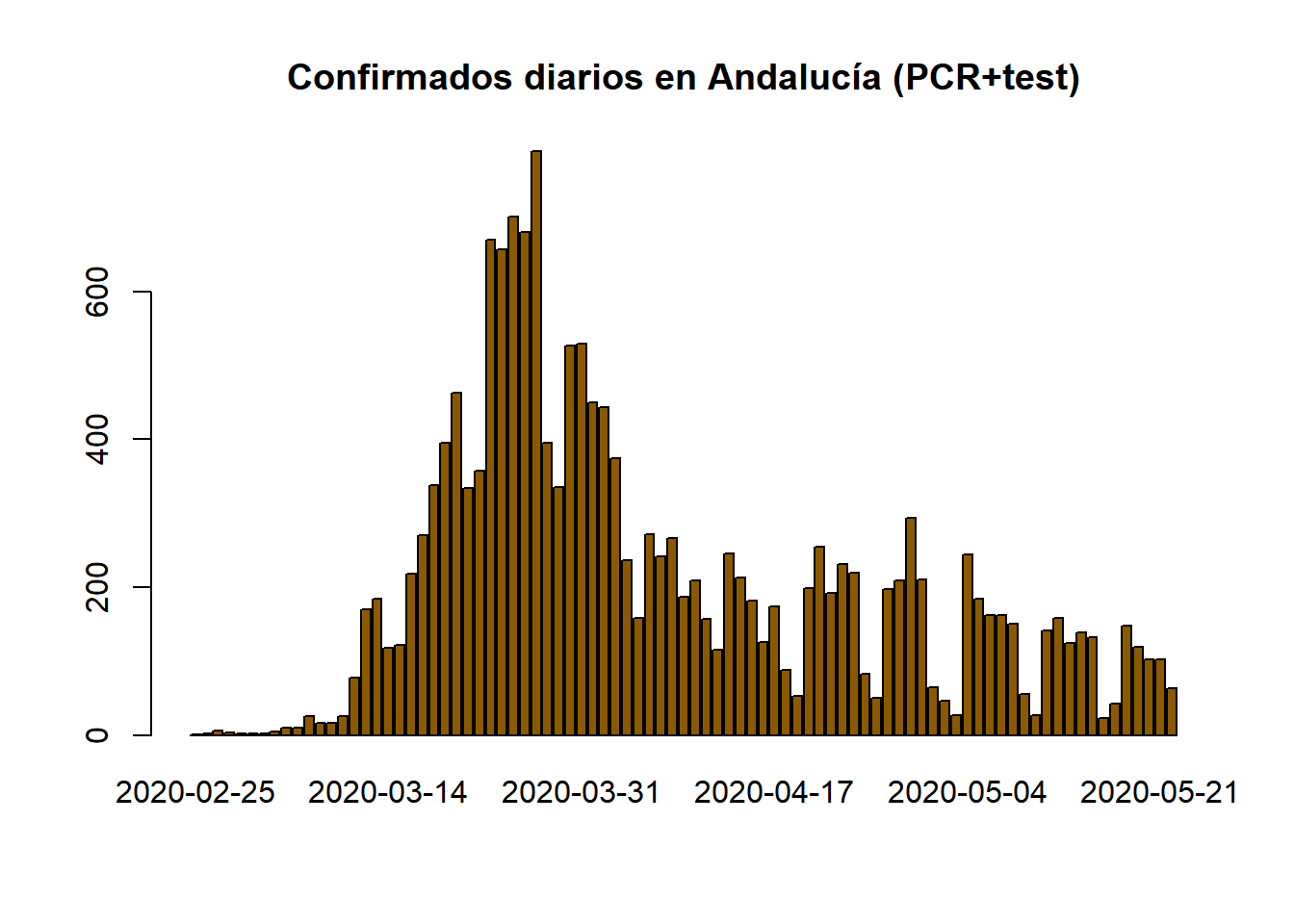
barplot(names.arg=aux$`Fecha declaración`,aux$`Total confirmados (PCR+test)`,ylim=c(0,max(aux$`Total confirmados (PCR+test)`)),main="Confirmados diarios en Andalucía (PCR+test)",col="orange4")
Map of Andalusia
# para manipular dataframes
library(tidyverse)
# para importar archivos shapefiles y excel
library(rgdal)
library(readxl)
# Para transformar los archivos shapefiles
library(broom)
library(ggplot2)
library(plotly)
# Guardamos el archivo shapefile
shapefile_provincias <- rgdal::readOGR("Provincias_ETRS89_30N/Provincias_ETRS89_30N.shp")
## OGR data source with driver: ESRI Shapefile
## Source: "C:\Users\Beatriz Huertas\Desktop\3º Ingeniería informática\2º cuatrimestre\Laboratorio de computación científica\Book covid analysis\Provincias_ETRS89_30N\Provincias_ETRS89_30N.shp", layer: "Provincias_ETRS89_30N"
## with 52 features
## It has 5 fields
# Para convertir el archivo shapefile en un dataframe utilizamos la función tidy()
data_provincias <- tidy(shapefile_provincias)
nombres_provincias <- data.frame(shapefile_provincias$Texto)
nombres_provincias$id <- as.character(seq(0, nrow(nombres_provincias)-1))
head(nombres_provincias)
## shapefile_provincias.Texto id
## 1 Ã\201lava 0
## 2 Albacete 1
## 3 Alicante 2
## 4 AlmerÃa 3
## 5 Ã\201vila 4
## 6 Badajoz 5
data_provincias_mapa <- left_join(data_provincias, nombres_provincias, by = "id")
reemplazos <-cbind(data_provincias,gsub("Almer�a","Almeria", data_provincias_mapa$shapefile_provincias.Texto)                   )
colnames(reemplazos)[8] <- "Provincias"
reemplazos$Provincias <- as.character(reemplazos$Provincias)
reemplazos$Provincias[2443:3298] <- "Almeria"
reemplazos$Provincias <- as.factor(reemplazos$Provincias)
provinciasandalucia <- filter(reemplazos,reemplazos$Provincias %in% c("Sevilla","Huelva","Córdoba","Málaga","Jaén","Almeria","Cádiz","Granada"))
cs_export <- read_excel("cs_export.xls") %>% print()
## # A tibble: 687 x 8
##    `Fecha declarac~ Territorio `Confirmados PC~ Hospitalizados   UCI Curados
##    <chr>            <chr>                 <dbl>          <dbl> <dbl>   <dbl>
##  1 22/05/2020       Andalucía                 9              6     0      26
##  2 22/05/2020       Almería                   1              2     0       4
##  3 22/05/2020       Córdoba                   0              0     0       1
##  4 22/05/2020       Granada                   0              1     0      11
##  5 22/05/2020       Huelva                    1              1     0       0
##  6 22/05/2020       Jaén                      5              2     0       1
##  7 22/05/2020       Málaga                    2              0     0       5
##  8 22/05/2020       Sevilla                   0              0     0       4
##  9 21/05/2020       Andalucía                16              5     0      52
## 10 21/05/2020       Almería                   0              0     0       4
## # ... with 677 more rows, and 2 more variables: Defunciones <dbl>, `Total
## #   confirmados (PCR+test)` <dbl>
# proceso los datos a utlizar
confirmados <-
  cs_export %>%
  group_by(Territorio, `Fecha declaración`)%>%
  print()
## # A tibble: 687 x 8
## # Groups:   Territorio, Fecha declaración [686]
##    `Fecha declarac~ Territorio `Confirmados PC~ Hospitalizados   UCI Curados
##    <chr>            <chr>                 <dbl>          <dbl> <dbl>   <dbl>
##  1 22/05/2020       Andalucía                 9              6     0      26
##  2 22/05/2020       Almería                   1              2     0       4
##  3 22/05/2020       Córdoba                   0              0     0       1
##  4 22/05/2020       Granada                   0              1     0      11
##  5 22/05/2020       Huelva                    1              1     0       0
##  6 22/05/2020       Jaén                      5              2     0       1
##  7 22/05/2020       Málaga                    2              0     0       5
##  8 22/05/2020       Sevilla                   0              0     0       4
##  9 21/05/2020       Andalucía                16              5     0      52
## 10 21/05/2020       Almería                   0              0     0       4
## # ... with 677 more rows, and 2 more variables: Defunciones <dbl>, `Total
## #   confirmados (PCR+test)` <dbl>
almeria <- confirmados %>% filter(Territorio=="Almería")
almeriaacum <- colSums(almeria[3:8])
cadiz <- confirmados %>% filter(Territorio=="Cádiz")
cadizacum <- colSums(cadiz[3:8])
cordoba <- confirmados %>% filter(Territorio=="Córdoba")
cordobaacum <- colSums(cordoba[3:8])
granada <- confirmados %>% filter(Territorio=="Granada")
granadaacum <- colSums(granada[3:8])
huelva <- confirmados %>% filter(Territorio=="Huelva")
huelvaacum <- colSums(huelva[3:8])
jaen <- confirmados %>% filter(Territorio=="Jaén")
jaenacum <- colSums(jaen[3:8])
malaga <- confirmados %>% filter(Territorio=="Málaga")
malagaacum <- colSums(malaga[3:8])
sevilla <- confirmados %>% filter(Territorio=="Sevilla")
sevillaacum <- colSums(sevilla[3:8])
dfaux <- data.frame("Provincia"=c("Sevilla","Málaga","Jaén","Huelva","Granada","Córdoba","Cádiz","AlmerÃ�a"),"Confirmados"=c(sevillaacum[6],malagaacum[6],jaenacum[6],huelvaacum[6],granadaacum[6],cordobaacum[6],cadizacum[6],almeriaacum[6]),"Hospitalizados"=c(sevillaacum[2],malagaacum[2],jaenacum[2],huelvaacum[2],granadaacum[2],cordobaacum[2],cadizacum[2],almeriaacum[2]),"Curados"=c(sevillaacum[4],malagaacum[4],jaenacum[4],huelvaacum[4],granadaacum[4],cordobaacum[4],cadizacum[4],almeriaacum[4]),"Defunciones"=c(sevillaacum[5],malagaacum[5],jaenacum[5],huelvaacum[5],granadaacum[5],cordobaacum[5],cadizacum[5],almeriaacum[5]))
dfaux$id <- as.character(c(40,28,22,20,17,13,10,3))
confirmadosmapa <- provinciasandalucia %>%
  left_join(dfaux, by= "id")
mapa <- confirmadosmapa %>%
  ggplot(aes(x=long, y= lat, group = group)) +
  geom_polygon(aes(fill=Confirmados), color= "white", size = 0.2) +
  labs( title = "Tasa de Contagios por Provincia",
        fill = "") +
  theme_minimal() +
  theme(
    axis.line = element_blank(),
    axis.text = element_blank(),
    axis.title = element_blank(),
    axis.ticks = element_blank(),
    plot.background = element_rect(fill = "snow", color = NA),
    panel.background = element_rect(fill= "snow", color = NA),
    plot.title = element_text(size = 16, hjust = 0),
    plot.subtitle = element_text(size = 12, hjust = 0),
    plot.caption = element_text(size = 8, hjust = 1),
    legend.title = element_text(color = "grey40", size = 8),
    legend.text = element_text(color = "grey40", size = 7, hjust = 0),
    legend.position = c(0.93, 0.3),
    plot.margin = unit(c(0.5,2,0.5,1), "cm")) +
  scale_fill_gradient(low = "yellow", high = "red")
ggplotly(mapa) %>%
  layout(title = 'Tasa de Contagios por Provincia')
## Hospitalizados
mapa <- confirmadosmapa %>%
  ggplot(aes(x=long, y= lat, group = group)) +
  geom_polygon(aes(fill=Hospitalizados), color= "white", size = 0.2) +
  labs( title = "Tasa de Hospitalizados por Provincia",
        fill = "") +
  theme_minimal() +
  theme(
    axis.line = element_blank(),
    axis.text = element_blank(),
    axis.title = element_blank(),
    axis.ticks = element_blank(),
    plot.background = element_rect(fill = "snow", color = NA),
    panel.background = element_rect(fill= "snow", color = NA),
    plot.title = element_text(size = 16, hjust = 0),
    plot.subtitle = element_text(size = 12, hjust = 0),
    plot.caption = element_text(size = 8, hjust = 1),
    legend.title = element_text(color = "grey40", size = 8),
    legend.text = element_text(color = "grey40", size = 7, hjust = 0),
    legend.position = c(0.93, 0.3),
    plot.margin = unit(c(0.5,2,0.5,1), "cm")) +
  scale_fill_gradient(low = "green", high = "red")
ggplotly(mapa) %>%
  layout(title = 'Tasa de Hospitalizados por Provincia')
## Curados
mapa <- confirmadosmapa %>%
  ggplot(aes(x=long, y= lat, group = group)) +
  geom_polygon(aes(fill=Curados), color= "white", size = 0.2) +
  labs( title = "Tasa de Curados por Provincia",
        fill = "") +
  theme_minimal() +
  theme(
    axis.line = element_blank(),
    axis.text = element_blank(),
    axis.title = element_blank(),
    axis.ticks = element_blank(),
    plot.background = element_rect(fill = "snow", color = NA),
    panel.background = element_rect(fill= "snow", color = NA),
    plot.title = element_text(size = 16, hjust = 0),
    plot.subtitle = element_text(size = 12, hjust = 0),
    plot.caption = element_text(size = 8, hjust = 1),
    legend.title = element_text(color = "grey40", size = 8),
    legend.text = element_text(color = "grey40", size = 7, hjust = 0),
    legend.position = c(0.93, 0.3),
    plot.margin = unit(c(0.5,2,0.5,1), "cm")) +
  scale_fill_gradient(low ="aquamarine", high = "darkblue")
ggplotly(mapa) %>%
  layout(title = 'Tasa de Curados por Provincia')
## Defunciones
mapa <- confirmadosmapa %>%
  ggplot(aes(x=long, y= lat, group = group)) +
  geom_polygon(aes(fill=Defunciones), color= "white", size = 0.2) +
  labs( title = "Tasa de Defunciones por Provincia",
        fill = "") +
  theme_minimal() +
  theme(
    axis.line = element_blank(),
    axis.text = element_blank(),
    axis.title = element_blank(),
    axis.ticks = element_blank(),
    plot.background = element_rect(fill = "snow", color = NA),
    panel.background = element_rect(fill= "snow", color = NA),
    plot.title = element_text(size = 16, hjust = 0),
    plot.subtitle = element_text(size = 12, hjust = 0),
    plot.caption = element_text(size = 8, hjust = 1),
    legend.title = element_text(color = "grey40", size = 8),
    legend.text = element_text(color = "grey40", size = 7, hjust = 0),
    legend.position = c(0.93, 0.3),
    plot.margin = unit(c(0.5,2,0.5,1), "cm")) +
  scale_fill_gradient(low ="gray46", high = "gray8")
ggplotly(mapa) %>%
  layout(title = 'Tasa de Defunciones por Provincia')